
Production Planning and Control (PPC): Functions and Examples
 User Solutions Team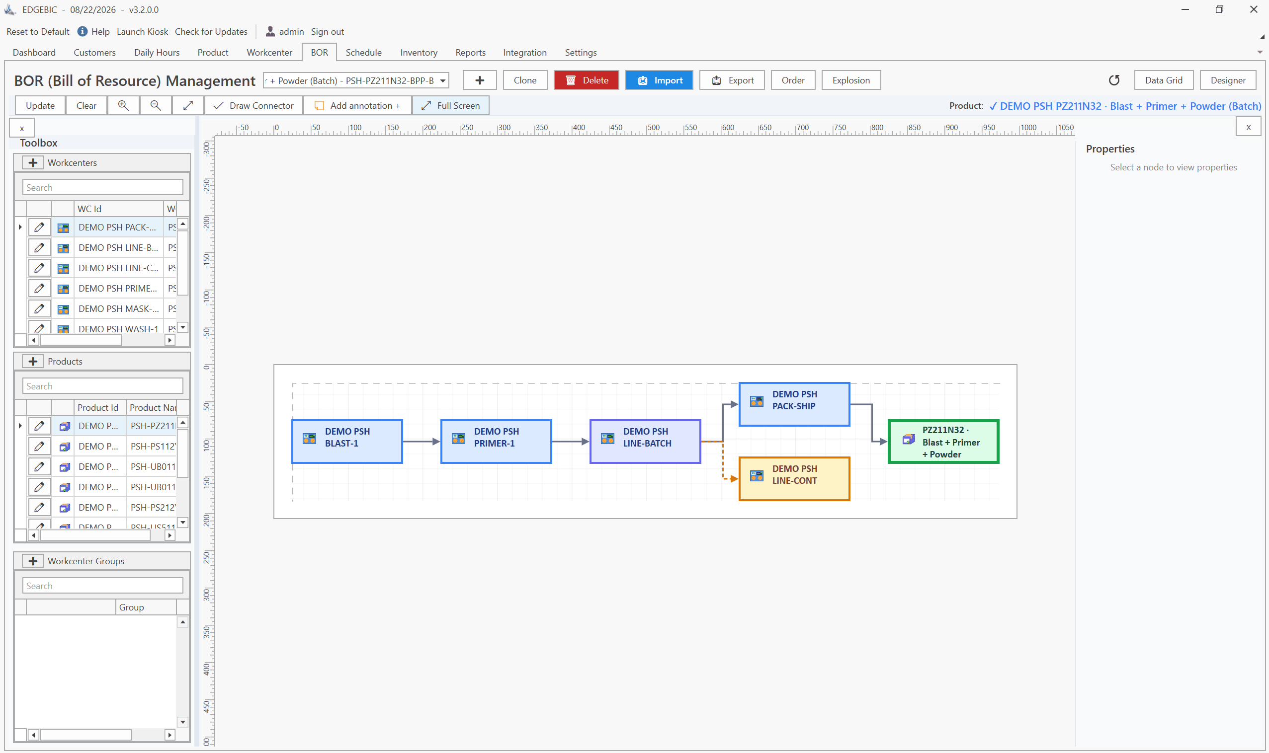
Production planning and control (PPC) is the system a factory uses to decide what to make, how, where and when (planning), and then to release the work, track it and correct the gaps (control). Its classic functions are routing, loading, scheduling, sequencing, dispatching and expediting. Textbooks describe them as a list. On a real shop floor they are a loop that runs every day.
Written by User Solutions, Inc., makers of RMDB and EDGEBIC (RMDB 2.0) by User Solutions, production planning and scheduling software for manufacturers since 1991. Reviewed by the User Solutions planning team. Updated September 2026.
This guide walks through each function with a worked example you can check by hand, then covers the types of scheduling in production planning and control. It is written for the planner, scheduler or operations manager who has to make it work, not for an exam.
PPC at a glance
| Phase | Function | Question it answers | Output |
|---|---|---|---|
| Planning | Routing | Which operations, on which work centers, in what order? | Routing with setup and run times |
| Planning | Loading | Is there enough capacity at each work center? | Load vs capacity by work center and period |
| Planning | Scheduling | When does each job start and finish? | Start and finish dates or times |
| Planning | Sequencing | In what order do jobs run at each work center? | Priority order per work center |
| Control | Dispatching | What does each work center do next? | Released work orders, dispatch lists |
| Control | Expediting (follow-up) | Which jobs are behind, and why? | Actions on late jobs |
| Control | Evaluation and corrective action | Did the plan work? What changes? | Metrics, updated parameters |
Above all of it sits the production plan: which products, how many, in which week. That comes from the sales and operations plan and the master production schedule, and MRP turns it into material orders (see what is MRP). PPC takes those quantities and makes them happen on the floor.
Planning versus control
The split matters because the two halves fail in different ways.
- Planning without control produces a schedule nobody follows. The Gantt chart looks perfect on Monday and is fiction by Wednesday.
- Control without planning is firefighting. Supervisors expedite whoever shouts loudest, and the plant is always busy and always late.
A working PPC system connects them: control feeds actual progress back into planning, and the next plan starts from what really happened. For the control half in more depth, read production control.
Function 1: Routing
Routing defines the path a part takes: the operations, the work center for each, and the setup and run times. It is the foundation for everything that follows, because loading and scheduling are only as accurate as the hours on the routing.
Worked example. A bracket, ordered in a quantity of 200:
| Op | Work center | Setup hours | Run hours per piece | Hours for 200 pieces |
|---|---|---|---|---|
| 10 | Saw | 0.50 | 0.02 | 0.50 + 4.00 = 4.50 |
| 20 | Mill | 1.50 | 0.10 | 1.50 + 20.00 = 21.50 |
| 30 | Deburr | 0.00 | 0.03 | 0.00 + 6.00 = 6.00 |
| 40 | Inspect | 0.25 | 0.01 | 0.25 + 2.00 = 2.25 |
| Total | 34.25 |
Operation hours = setup hours + (run hours per piece x quantity)
Two practical points. First, the mill is 21.5 of the 34.25 hours (63 percent), so the mill will decide when this order ships. Second, setup is spread over the lot: at 50 pieces, the mill would need 1.5 + 5.0 = 6.5 hours, and setup would be 23 percent of it instead of 7 percent. Lot size is a routing decision too. See what a routing is and how a routing graph orders steps for scheduling.
Function 2: Loading
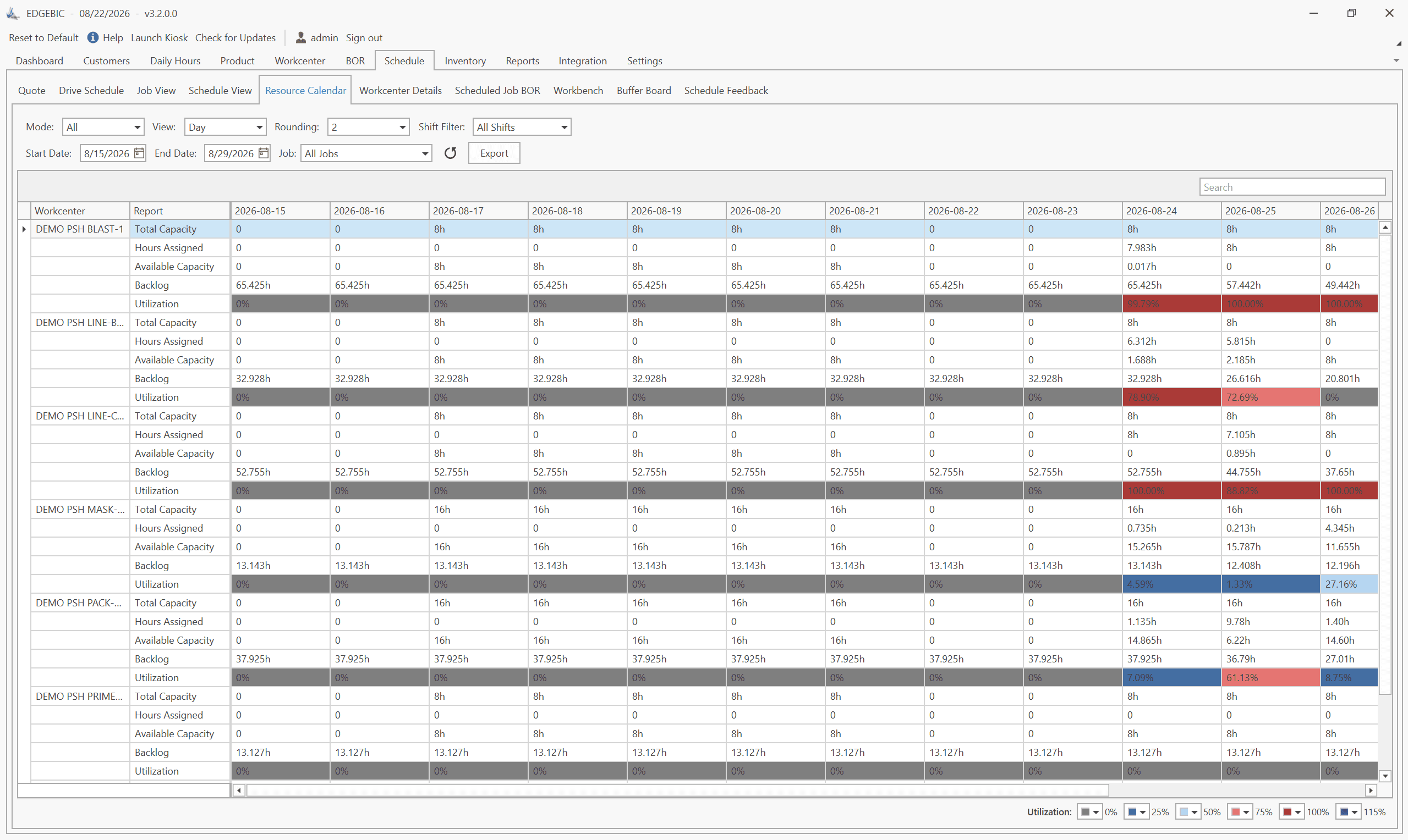
Loading assigns the hours from every routing to work centers for a period, then compares them with capacity. It tells you whether the week is possible before you spend time sequencing it.
Load % = hours assigned to the work center / available hours x 100
Worked example. One week's load:
| Work center | Available hours | Loaded hours | Load | Status |
|---|---|---|---|---|
| Saw | 40 | 32 | 80% | OK |
| Mill (2 shifts) | 80 | 94 | 118% | Over by 14 hours |
| Lathe | 40 | 30 | 75% | OK |
| Weld | 40 | 38 | 95% | Tight |
The mill is over by 14 hours (94 - 80). No sequence can fix that; only hours can. The planner's options: 8 hours of Saturday overtime, plus moving a 6-hour job with a later due date into next week (8 + 6 = 14). The lathe's spare 10 hours do not help unless some mill work can run on the lathe, which is why routings should list alternate work centers where they exist.
Loading that ignores capacity (infinite loading) only reports the 118 percent. Finite loading refuses to put more than 80 hours on the mill and pushes the excess out, showing which jobs move. See loading and finite vs infinite capacity scheduling. To run a weekly load check yourself, use the free capacity planning Excel template.
Function 3: Scheduling
Scheduling sets the start and finish time of each job, operation by operation, inside the capacity that loading confirmed. Two directions:
- Forward scheduling starts each job as soon as possible and calculates the finish. It answers "when is the earliest we can ship?"
- Backward scheduling starts from the due date and works back, so each operation starts as late as possible. It keeps work-in-process and raw material low.
Most plants use forward scheduling to find what is late and backward scheduling for jobs with slack. See forward vs backward scheduling. For a step-by-step build with a free template, read how to create a production schedule.
Function 4: Sequencing
Sequencing decides the order of jobs at each work center. With the same total hours, a different order produces very different lateness.
Worked example. Four jobs wait at one machine at the start of day 0. Processing time and due day:
| Job | Processing days | Due day |
|---|---|---|
| A | 6 | 8 |
| B | 2 | 6 |
| C | 8 | 18 |
| D | 3 | 15 |
Three common rules, each finishing all 19 days of work:
| Rule | Order | Completion days | Days late per job | Total days late | Jobs late | Average flow time |
|---|---|---|---|---|---|---|
| First come, first served | A, B, C, D | 6, 8, 16, 19 | 0, 2, 0, 4 | 6 | 2 | 49 / 4 = 12.25 |
| Shortest processing time | B, D, A, C | 2, 5, 11, 19 | 0, 0, 3, 1 | 4 | 2 | 37 / 4 = 9.25 |
| Earliest due date | B, A, D, C | 2, 8, 11, 19 | 0, 0, 0, 1 | 1 | 1 | 40 / 4 = 10.00 |
Reading it: shortest processing time gets jobs through fastest on average; earliest due date cuts lateness from 6 days to 1. First come, first served, which is what most shops do by default, is worst on both. Real sequencing also weighs setups (running similar jobs together) and customer priority. See priority rules, job sequencing and critical ratio scheduling.
Function 5: Dispatching
Dispatching turns the schedule into action. It releases the work order, and makes sure the materials, drawings, tooling and program are at the work center when the job is due to start. Each work center gets a dispatch list: its jobs, in order, with start times.
Good dispatching has three rules:
- Release only what can run. A job released without material just becomes queue.
- One list per work center, one version. If supervisors keep their own lists, the schedule is advice, not a plan.
- Refresh it every shift. When a job finishes early or late, the list updates.
See dispatch list and how a dispatch list replaces the loudest voice.
Function 6: Expediting (follow-up)
Expediting, also called follow-up or progress chasing, tracks jobs against the schedule and clears whatever blocks the late ones: a missing part, a down machine, a quality hold, a lost traveler.
A little expediting is normal. A lot is a symptom. If most jobs need chasing, the plan was not feasible to begin with, usually because loading was never checked or sequence was left to the floor. The fix is upstream, in functions 2 to 4, not in more expeditors. See how EDGEBIC reduces expediting.
Function 7: Evaluation and corrective action
The loop closes by measuring what happened and fixing the parameters that caused the gaps:
| Metric | Formula | What a bad number points to |
|---|---|---|
| Schedule adherence | Jobs finished in their scheduled period / jobs scheduled x 100 | Unrealistic capacity, poor dispatching |
| On-time delivery | Orders shipped by the promise date / orders shipped x 100 | Loading or sequencing problems |
| Load vs capacity | Loaded hours / available hours by work center | Chronic bottleneck, wrong available hours |
| Routing accuracy | Actual hours / standard hours by operation | Bad routing data |
Update the routings, the available hours and the sequencing rules from what the numbers show, and the next plan starts closer to reality. For the full metric set, see production scheduling KPIs.
Types of scheduling in production planning and control
Scheduling is classified several ways. A real plant uses more than one at once.
By level
- Master scheduling: end items by week, over months. See what is a master production schedule.
- Operations (detailed) scheduling: each operation on each work center, by hour or minute, over days or weeks.
By direction
- Forward scheduling: start as soon as possible; finish date is the result.
- Backward scheduling: start from the due date; start date is the result. See backward scheduling.
By capacity
- Infinite capacity scheduling: ignores what else is on the work center. Simple, often wrong in a busy plant. This is what MRP does; see MRP vs APS.
- Finite capacity scheduling: respects real hours, shifts and existing load.
By production system
| System | Typical products | Scheduling focus |
|---|---|---|
| Job shop | Custom, high-mix, low-volume | Sequencing many different routings through shared machines |
| Batch | Families of similar products | Lot sizes and changeovers |
| Flow or line | High-volume, standard products | Line balancing and rate |
| Project | One-off large builds | Activity networks and milestones |
By trigger
- Push: work is released according to the schedule.
- Pull: work is released when downstream consumes, as with kanban.
For how the main methods compare, read production scheduling methods.
PPC in a small or mid-size plant
Large manufacturers run PPC across several systems and a planning department. A 50-person shop runs it with one planner, an ERP or accounting system, and usually Excel. The functions are the same; the tools are lighter.
A practical setup that works:
- Plan quantities in the ERP's MRP or with the factory production planning template.
- Route, load, schedule and sequence in a finite capacity scheduler, or in the production schedule Excel template while the shop is small.
- Dispatch with one printed or on-screen list per work center.
- Follow up daily: record what finished, reschedule, republish.
- Review monthly: adherence, on-time delivery, routing accuracy.
EDGEBIC (RMDB 2.0) by User Solutions covers steps 2 to 4 beside any ERP. It models routings with a graphical routing editor, loads and schedules every operation against finite capacity and shift calendars, sequences with setup matrices and optimization, and produces Gantt charts and dispatch lists. It continues RMDB, the engine behind 35 years of User Solutions customer results, including GE Railcar Services, which raised on-time shipping from 30% to over 90%. EDGEBIC APS is $25,000 one-time; EDGEBIC Complete, which adds MRP, inventory and purchasing, is $35,000 one-time. See production scheduling software, EDGEBIC and pricing.
Related reading
Frequently Asked Questions
Ready to Transform Your Production Scheduling?
User Solutions has been helping manufacturers optimize their production schedules for over 35 years. One-time license, 5-day implementation.

User Solutions Team
Manufacturing Software Experts
User Solutions has been developing production planning and scheduling software for manufacturers since 1991. Our team combines 35+ years of manufacturing software expertise with deep industry knowledge to help factories optimize their operations.
Share this article
Related Articles
How to Create a Production Schedule in 7 Steps (Free Template)
How to create a production schedule step by step: horizon, real capacity, work orders, load check, sequence, dates, then publish. Worked example included.

Sequence-Dependent Setup Times: The Scheduling Problem That Costs You Capacity
When changeover time depends on what ran before, standard scheduling fails. Learn how setup matrices, sequence optimization, and APS software recover 10-25% of hidden capacity in paint lines, food, and coating operations.

Subcontracting in Your Production Schedule: When and How to Outsource Operations
Learn how subcontracting changes your production schedule - modeling OP lead times, outside processing routing steps, vendor capacity constraints, and single-source subcontractor risk.