What Is a Master Production Schedule (MPS)?

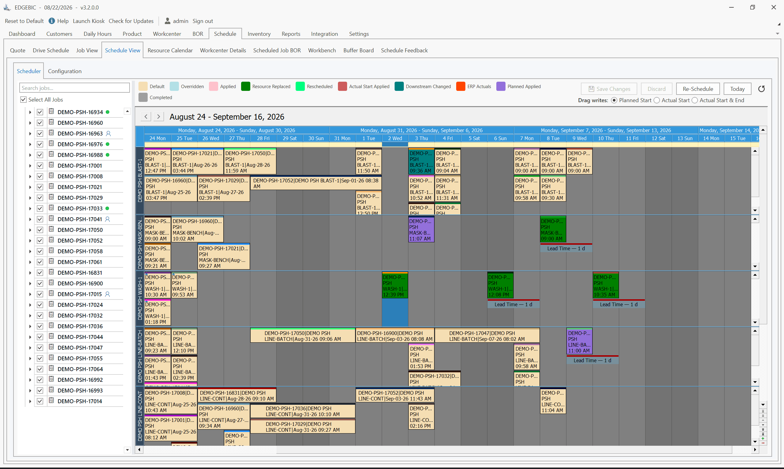
A master production schedule (MPS) is a planner-committed, time-phased build schedule for finished goods, sitting between raw demand and the detailed material and capacity plan. It answers a specific question for each finished item: how many should we build in each time bucket. Crucially, it is a human decision rather than an automatic output. A planner weighs projected demand against inventory and capacity, then commits a build quantity per period. That committed plan drives everything downstream, from material netting to shop floor scheduling.

This entry defines the MPS and shows how it behaves inside EDGEBIC by User Solutions. For the wider index of planning terms, see the manufacturing glossary, and for the period structure an MPS is built on, read what is a master production schedule bucket.

How it works

The everyday version of an MPS is a bakery manager's weekly board: "Monday, 200 sourdough and 100 baguette; Tuesday, 300 sourdough." Those numbers are not guesses generated by a spreadsheet. They are decisions the manager makes after looking at pre-orders, the usual walk-in average, and how much flour is on hand. The board is the master schedule for the bakery's finished goods.

An MPS is time-phased, meaning it spreads committed quantities across a series of buckets, usually weeks or custom periods. Each cell is one product in one bucket with a committed build quantity. Because the plan is explicit and forward-looking, a planner can see where capacity gets tight, where a demand spike lands, and where inventory will run thin, and adjust the committed quantities before problems reach the floor.

The commitment happens in stages so the plan can stay soft while it is being shaped, then lock when the planner is ready. A suggested quantity is one the system calculated but the planner has not confirmed. A firm quantity is one the planner has committed to but has not yet turned into a work order. A released quantity is one that has become a real build order, which then acts as the scheduled supply feeding the finite capacity schedule.

A concrete example

A make-to-stock bracket sells steadily, and the planner keeps a projected inventory view week by week. In week 14, projected demand is 100 and projected stock would dip below the safety level, so the system suggests building 100. The planner reviews it, agrees, and firms the bucket at 100. Nothing has been built yet, but the commitment is on record.

Later, ready to execute, the planner releases that week-14 firm entry. A build-to-stock work order for 100 units due in week 14 is created, and it becomes the scheduled receipt that lifts projected inventory back above the safety line. If the shop scraps 2 units during the run, the order completes and posts a receipt of 98, and the planner sees the 2-unit shortfall against the 100 committed, a small signal to watch yield on that item.

How EDGEBIC uses it

In EDGEBIC, the master production schedule is a working screen where a planner overlays committed build quantities on top of the projected inventory picture for each finished item. Each master schedule entry carries a product, a bucket, a bucket date, and a committed quantity, and it moves through the suggested, firm, and released stages as the planner decides and acts.

Firming an entry records the planner's commitment without creating any work. Releasing a firm entry atomically creates a build-to-stock manufacturing order and stamps the entry with that order's reference, so the master schedule and the shop floor stay linked. From that point the released order flows into the scheduling engine as a real demand, gets placed onto work centers within their finite capacity, and completes with a real inventory receipt.

Because EDGEBIC is a scheduling and planning specialist rather than a full ERP, the demand and item data behind the MPS arrive through flexible Excel, CSV, and database import and export masks. That lets the master schedule reflect whatever forecast and order data your business already keeps, without requiring a native connector to any single ERP.

To understand the bucket structure the MPS lays quantities into, continue with what is a master production schedule bucket. For the calculation that explodes committed finished-goods quantities into component needs, read what is capacity requirements planning. And for the broader system that turns a committed plan into a runnable schedule, see what is advanced planning and scheduling.